It’s no secret that manual data entry is both a grueling and slow process. Slow data entry means that the information those documents contain takes time to flow down a company’s pipeline.
Let’s imagine our client is a supply chain company. This client is dealing with a large amount of invoices from a diverse pool of providers. Diverse providers prohibit the company from simply automatizing the invoice data entry process because each provider uses a different and unique template. Hyperscience eliminates that bottleneck by automating data entry using state of the art artificial intelligence.
In this blog post, we will showcase how pointer networks can be leveraged to confidently extract the required information from a dozen templates and a small amount of labeled data, a core value of the Hyperscience Platform.
What is a Pointer Network?
Pointer networks are a Deep Learning model which can learn how to select specific items of an object sequence using supervised learning. This architecture deals with the fundamental problem of representing variable length dictionaries by using a softmax probability distribution as a “pointer1.”
An example of pointer networks in action can be seen within the traveling salesman problem (TSP). The traveling salesman problem is a typical problem of modern combinatorial mathematics and is often formulated through a city metaphor. Given a set of cities and distance between every pair of cities, the problem is to find the shortest possible route that visits every city exactly once and returns to the starting point2.
The traveling salesman problem is part of the subset of NP-hard problems3. It’s a very hard class of combinatorial problems, for which at this point there is no known solution with polynomial runtime, and may very well never have one. This means that those problems can take a really long time to solve, especially as the number of input increases.
When faced with such a problem, it is critical to find good approximations in polynomial time. Pointer networks can be used to do just that using Deep Learning. It’s a very interesting instance of Deep Learning helping to solve theoretical mathematical problems.
Solving Combinatorial Problems with Deep Learning
A Pointer network is made up of three main components:
- The encoder
- The decoder
- The attention module
A simplified version of the traveling salesman problem can be formulated as follows:
Input: Cities are points with coordinates in [0, 1]*[0, 1]
Output: The permutation of cities representing the optimal path on this fully connected graph
First, we format the coordinates of the cities as a vector which we call

Then, we feed this sequence of vectors to the encoder (typically a RNN) and we recover an embedding for each vector, as well as the last hidden state of the encoder.
That last hidden state is then fed to the decoder, which outputs a vector that we will call a query. That query is then compared to each embedding outputted by the encoder by leveraging the attention module.
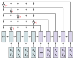
The input embedding that scores the highest will be retained as the first city. We continue unrolling the decoder until it outputs the stop token.
With this approach, a quality approximation to the traveling salesman problem, was found using Deep Learning, with comparable or lower complexity. The model, once trained and decoded with a beam search constrained to find valid solutions, outputs tours of comparable length to approximate solutions found by two algorithms. The complexity of the pointer network is O(n2) and the two approximation algorithms are of complexity O(n2) and O(n3). For more details see section 4.4 of this paper.
How Are We Leveraging Pointer Networks?
The problem we are tackling here is extracting information from semi-structured documents. Here is how we classify three different types of documents:
- Structured documents: templates where we know exactly where the information is located
- Unstructured documents: free form text, typically a lot of dense paragraphs
- Semi-structured: the information is clearly labeled in the document but does not follow a specific structure
For that reason, it is important to look at the words and their 2D location within the document so that the model can understand the spatial context. We would lose this context if we looked at this problem as linear 1D text.
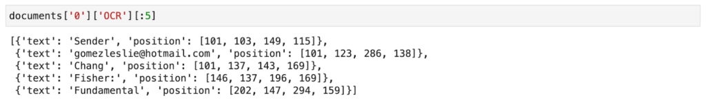
After extracting the text from the document with the OCR engine, we feed each of those words and positions to the pointer network. Then, we train it to output the sequence of a specific field we are looking for.
Let’s say we are looking for the sender address on a document.
First, we feed all of the document’s tokens to the pointer network encoder.
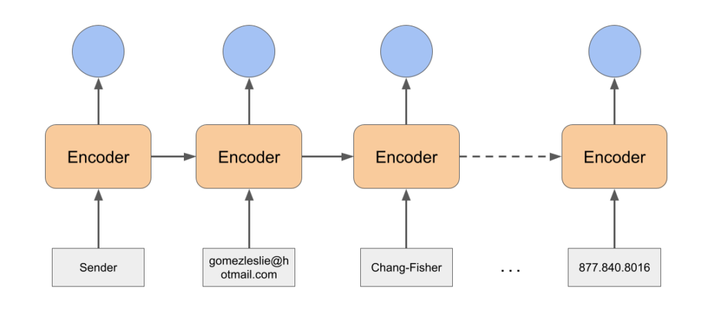
Once we have fed the entire sequence to the encoder, we retrieve the last hidden state. We will use it as the first input token to the decoder. Thanks to a simple attention mechanism, the decoder predicts one of the input tokens as the first token of the address.
Then, we feed the embedding for that token to the Pointer network, and the process continues.
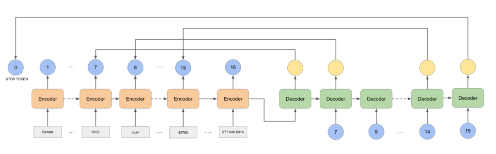
Now that we have a complete predicted sequence, we can back propagate on the PointerNetwork by penalizing it on finding the right sequence of words corresponding to the address.
Putting Theory into Practice
[AUTHOR’S NOTE] All of the following code and reproducible notebook can be found here.
Toy Dataset
A typical problem that we tackle at Hyperscience involves extracting information from invoices with many unseen templates. In order to generate a non-trivial and realistic dataset, we used the Python package Faker, along with randomisation of the location information and the surrounding context.
The information present include:
- The address and name of the company receiving the invoice
- The metadata of the invoice, i.e. date and identification number
- The address, phone number and email address and name of the company sending the invoice
- The content of the invoice, i.e. description, quantity and amount
That dataset contains only 1,000 documents, which is notoriously small when it comes to Machine Learning and even more so when training Deep Learning algorithms from scratch.
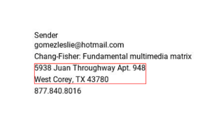
Example document:
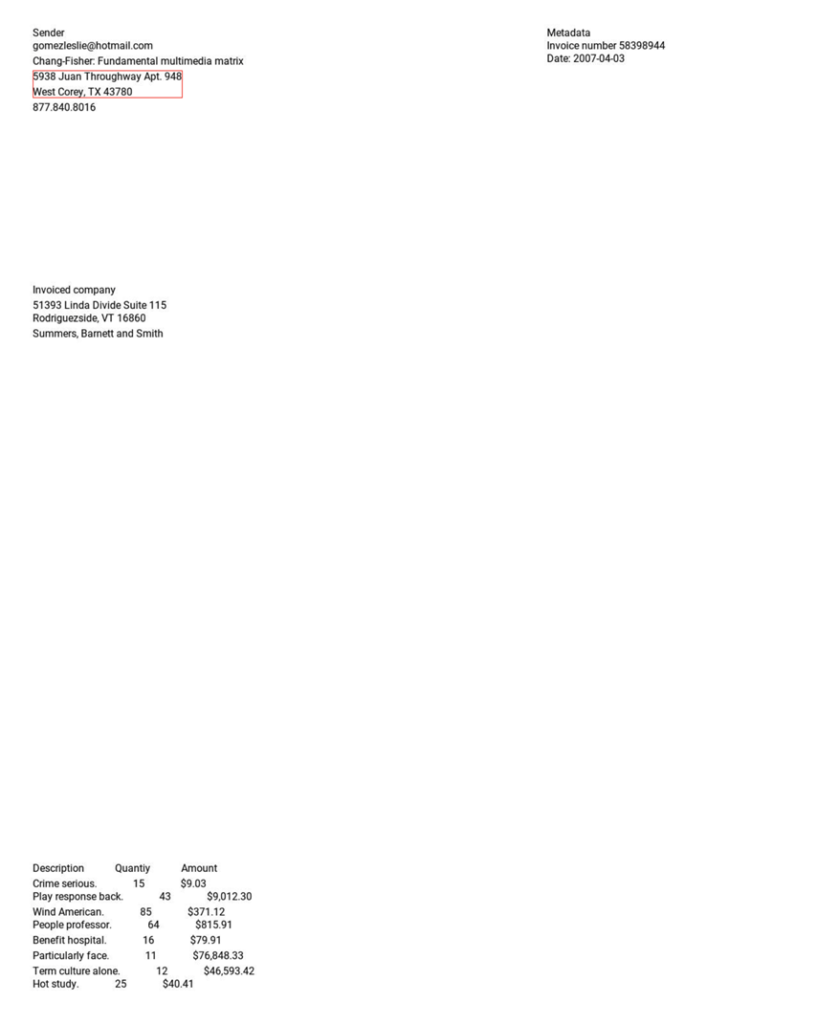
We show the position of the sender’s address we want to extract in red.
Pre-processing
As with all MachineLearning projects, the first step is to do some pre-processing. In our case, we must retrieve the text content out of the images of the document.
OCR with Tesseract
Tesseract is:
- A popular open source OCR4.
- Low on performance in non-perfect settings.
We use it here to show the end-to-end process and add realistic noise (i.e. transcription errors) to the data, which we have to deal with in a real life setting.
Labels
We know the location of the address on the document, however, we need to retrieve the indices of the corresponding tokens as extracted by pytesseract so we can train the Pointer network to find them.

Split Train / Validation / Test
As mentioned in the introduction, our goal is to automate data entry with high accuracy. In order to do so, we need to make high confidence decisions. A very typical way to calibrate that confidence is to optimize thresholds on the validation set and confirm that they work well on the test set.
For that reason we split our dataset with the following percentages 60 / 20 / 20. This means that we will be training the model on only 600 documents, and validating it on 200.
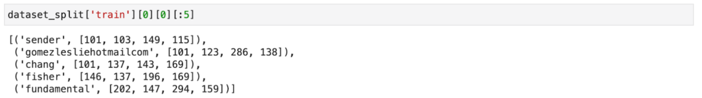
Cleaning the Text
When cleaning text for a NLP task, one has to keep in mind what kind of technique will be used to embed the words. For example, a pre-trained embedding (i.e. word2vec or fasttext) approach would require a fixed vocabulary and pre-training the word embedding prior to the model itself. Here, we are going to opt for an end-to-end architecture, which has the benefit of being simple to implement and will allow the model to learn the embeddings that benefit the end task most.
For this end-to-end approach, we will adopt a very simple architecture. First, we embed at the character level in order to have a small vocabulary for simplicity and be more resilient to OCR transcriptions errors. Then, we feed that sequence of vectors to a LSTM and finally retrieve the final hidden state as the word embedding. Because we plan on embedding at the character level, we should try and reduce the number of characters.
After cleaning the text, each page is stored as a list of tuples of words and their corresponding position on the page:
Getting the Data Ready for Training
In order to speed up training, we’ll want to have a batch_size greater than one. This requires us to put every example in tensor format so that we can batch them.
We have three types of vectors for this problem:
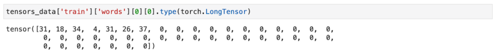
- The words on a page in character format:
- 0 is used for padding
- All characters the word are mapped to an integer
Thus the word ‘invoice’ is transformed into the following tensor:
- The position of each word on the page, we keep the same format as before:

- The target padded with 0s

When putting all of this together, we get three multidimensional tensors:
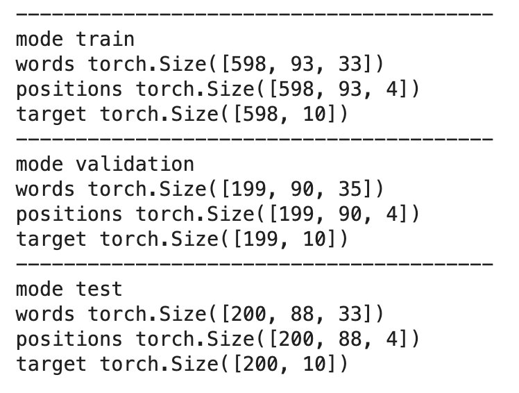
- Words
- First dimension = size of the dataset
- Second dimension = max number of words on any page
- Max number of characters in a word
- Positions:
- First dimension = size of the dataset
- Second dimension = max number of words on any page
- For values corresponding to x, y coordinates in pixels of the top left corner of the rectangle fitting the word followed by the x, y coordinates of the bottom left corner
- Targets:
- First dimension = size of the dataset
- Second dimension = max number of words in the target address
Modeling
We can break down the model in a couple of components:
- Word embedder
- Encoder
- Decoder
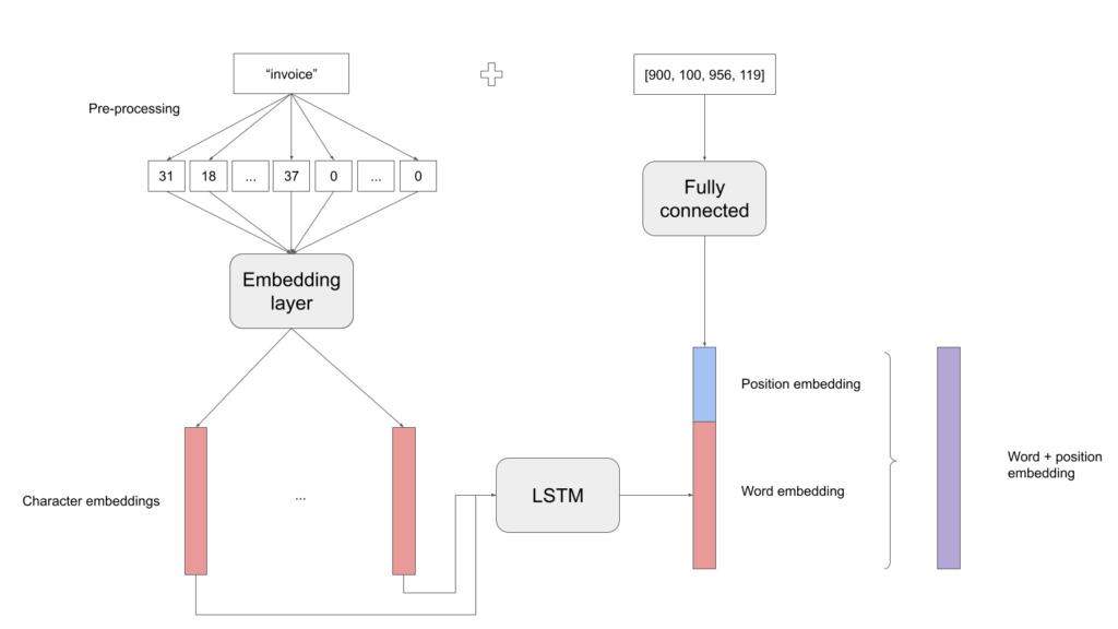
Word Embedder
As described before, our approach is relatively simple:
- First embed each character of the word with an Embedding Layer
- Feed them to a LSTM
- Retrieve the last hidden layer. This is your word embedding
Implementation in PyTorch
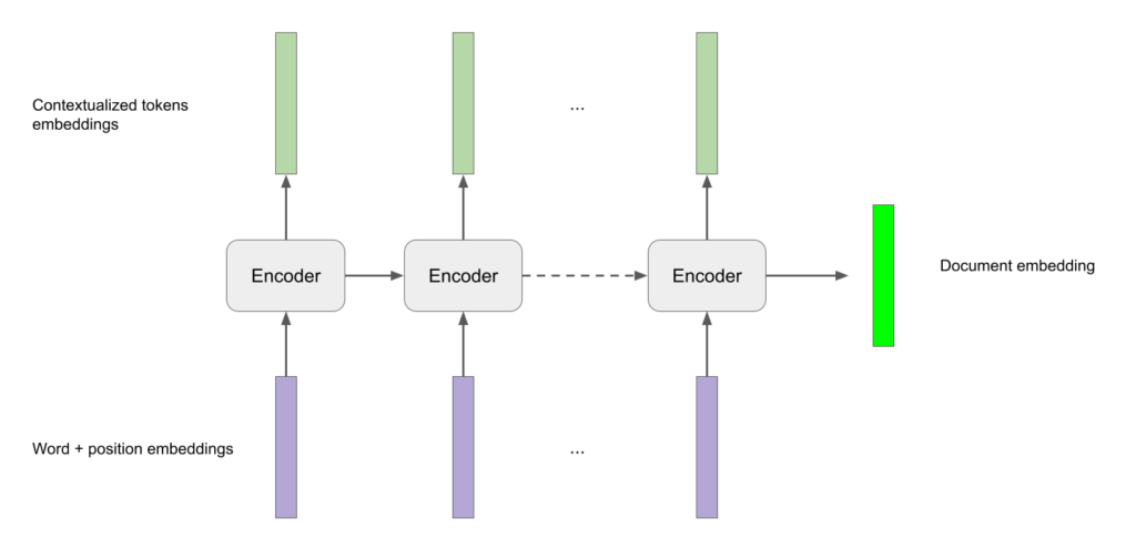
Encoder
The structure of the encoder is extremely simple. It’s a simple LSTM that inputs the sequence in reading order (left to right, top to bottom) of words and positions embeddings on a page from the word embedder step. It returns contextualized embeddings for each token along with the last hidden state that we will use as document embedding.
Implementation in PyTorch
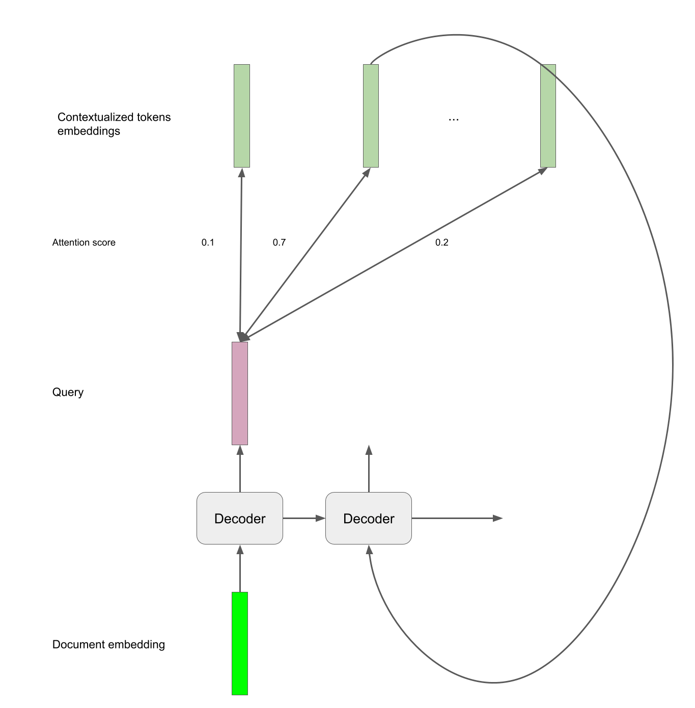
Decoder
The decoder is the other half of the Pointer network. We unroll a LSTM Cell and compare the outputted hidden states to the contextualized embeddings through the attention mechanism to find the correct tokens that are part of the address.
Implementation in PyTorch
Model
We put all of the above together and end up with the following implementation, with the words and their positions in input and in output the indices of the predicted sequence of token corresponding to the address along with their probabilities.
Implementation in PyTorch
Training Results
Training and Validation Loss
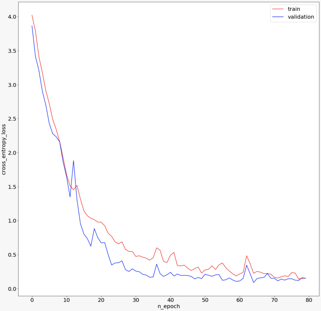
- Red signifies training loss
- Blue signifies validation loss
We have a quick decline of the loss at the beginning of training that converges towards a plateau around the 50th epoch. We do not observe overfitting thanks to the dropout we added to our multiple modules.
Validation Accuracy
Ultimately, we pick the trained model with the best validation accuracy.
Metrics and Automation
Confidence Score
All deep learning algorithms commit errors. It is essential to know when the model is likely to be wrong so we can lean on the help from a human to be as perfect as possible.
In order to do so, we devise a simple confidence score, which is simply the mean of the confidences on each token the Pointer network predicted.
Correct versus Incorrect Predictions
On this graph, we show the histogram of correct versus incorrect predictions on the validation set:
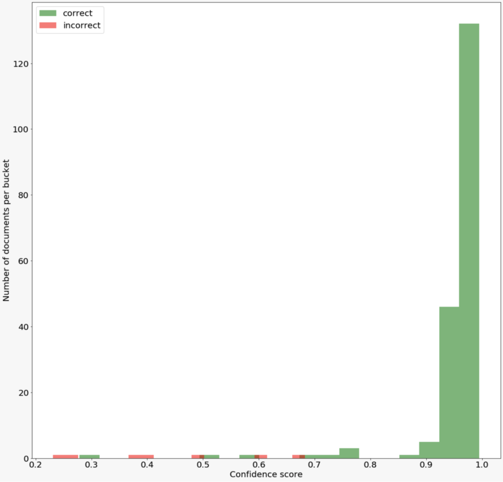
This is an ideal outcome. The model does not commit mistakes when the confidence score is high. It only commits mistakes when the score is low and the intersection of the tails of those two distributions is quite small. This means it will be easy to separate confident predictions from potential mistakes.
Automation
In order to make decisions with high accuracy, we look for a threshold on the validation dataset that allows us to reach 99% accuracy on predicted addresses.
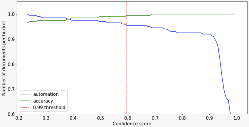
That threshold comes to 0.596. At that value, we get an accuracy of 99.5% and an automation of 95.4%. This means that 95.4% of the time we can find the address automatically and only make an error 0.05% of the time.
Next, we need to confirm those results on the test dataset to make sure we didn’t overfit that hyperparameter on validation. At the threshold 0.596 on the test dataset, we get 91.5% automation and 98.9% accuracy.
Conclusion
Summary of Results
| Accuracy | Automation | |
| Validation dataset | 99.5% | 95.4% |
| Test dataset | 98.9% | 91.5% |
The aforementioned data showcased the power of Pointer networks to extract information from semi-structured documents in low data regimes. Furthermore, we are able to get extremely high automation rates of 91.5 at 98.9% accuracy.
While this is a toy dataset, the variability we introduced with randomness makes it relatively realistic. Furthermore, this is a very simple implementation and we could improve performance within areas such as better word embeddings, ensembling and data augmentation.
As a reminder, all of the aforementioned code and reproducible notebook can be found on the Hyperscience GitHub.
Jocelyn Beauchesne is an ML Engineer at Hyperscience based out of our New York office. Connect with him on LinkedIn.