Introduction to Conditional Random Fields
This month’s Machine Learn blog post will focus on conditional random fields, a widely-used modeling technique for many NLP tasks. Conditional random fields (CRFs) are graphical models that can leverage the structural dependencies between outputs to better model data with an underlying graph structure.
If you have ever used an open-sourced implementation for CRFs, or if you take a look at an equivalent PyTorch implementation, you may have noticed that the torch module has a surprising workflow:
- The forward() method returns the log-likelihood of the input sequences.
- The inference is done via a `decode()` method, not via the forward method.
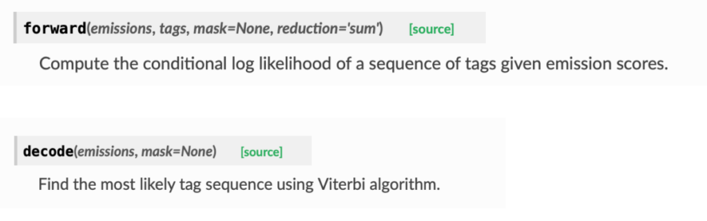
This unusual workflow is a direct consequence of the inner workings of CRFs.
Although CRFs can be used on arbitrary graphs, one of the main applications is NLP: any text can be modeled as a sequence (called linear chain), which is a special case of directed graphs. CRFs used for sequences are called linear-chain CRFs. In this article, we will focus on demystifying linear-chain CRFs, and demystify them. In the subsequent sections we will showcase:
- An example of applications with named-entity recognition (NER)
- A brief overview of the conditional distribution learned by a CRF
- The CRF loss, and the use of the forward-backward algorithm
- An explanation of the decode() method based on the Viterbi Algorithm
- Some limitations of CRFs in terms of document processing
[Author’s Note] In many different fields, like Physics or Statistics, a random field is the representation of a joint distribution for a given set of random observations. As we will see later, CRFs model the conditional probability distribution from a set of random observations, hence the name “conditional random field”.
CRF Applications
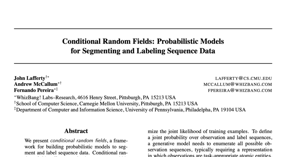
CRFs are used for a large array of tasks, including sequence classification tasks such as part-of-speech tagging or named-entity recognition. It was first presented in 2002, but it is still used for most of the SOTA implementations on major benchmark datasets. For instance, if you look at CONLL2003, you will see that the vast majority of models are using a BiLSTM-CRF layer (which is essentially a CRF on top of a Bi-LSTM layer) combined with a BERT encoder.
See below some stats on mentions to CRF.
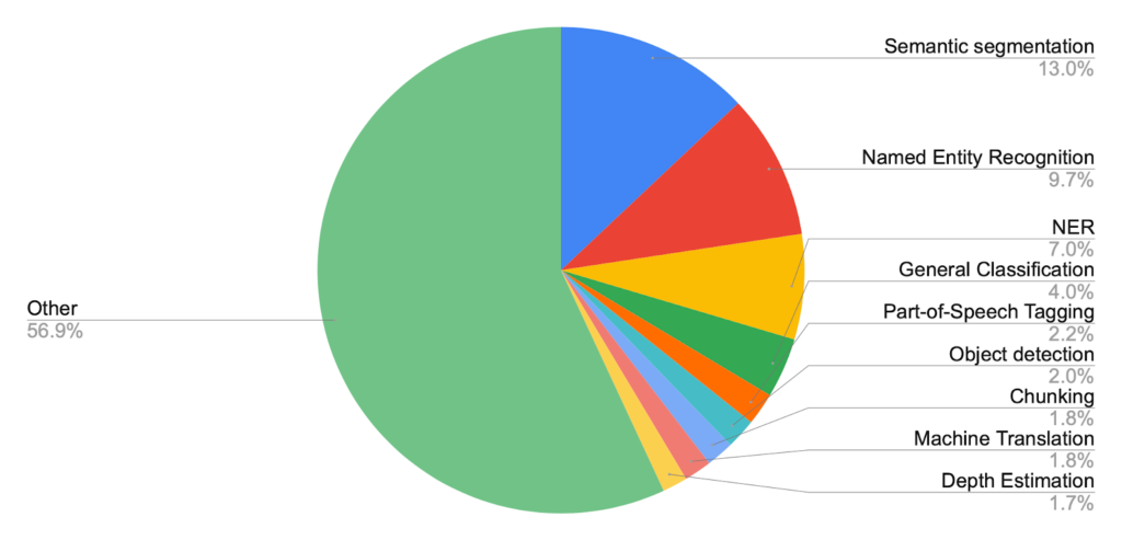
Source: Papers With Code https://paperswithcode.com/
For the remainder of the blog post, we will use named-entity recognition (NER) as an example for understanding how linear-chain CRFs work, but none of the technical points discussed will be specific to NER.
Insights into Named-Entity Recognition
The goal of NER is to retrieve named entities in a sequence of tokens (usually words). In the example below, the task is to extract location, person, and organization named entities. In practice, it consists of labeling each word in the sequence from a fixed set of class labels following a common IOB tagging format. In the illustration below, you can see B-ORG, O, B-MISC assigned to the tokens “EU”, “rejects” and “German”, respectively.Ultimately, NER is a multi-class classification problem, where we classify each token to the above-defined classes. This is usually referred to as sequence labeling.
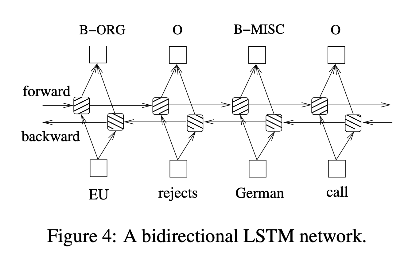
Source: Bidirectional LSTM-CRF Models for Sequence Tagging https://arxiv.org/pdf/1508.01991v1.pdf
For this sequence labeling task, linear-chain CRFs have shown great performance improvements out-of-the-box. In most cases, simply take your NER model, add a CRF to it, and results will improve.
In the next section, we will uncover some of the statistical explanations behind the performance improvement from CRFs.
A Statistical Look at CRFs
Without the CRF: Optimizing the Token Likelihood
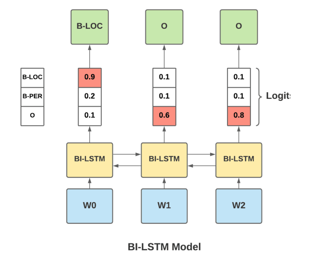
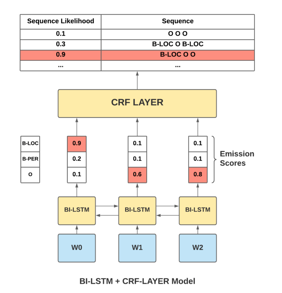
Imagine we use a Bi-LSTM model with some word embedding for our NER task (illustrated in the graph below). We obtain the logits per class for each word from the Bi-LSTM, but each prediction for a specific word is not dependent on the predictions of its neighbor. The model classifies each token while unaware of the predictions of the surrounding neighbor tokens.
In that case, we model the sequence conditional probability P(Y|X) as:
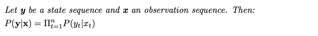
This means the conditional probability of the sequence Y is the product of the probabilities of each token in the sequence. This implies independence between the predictions; there is no interaction between labels.
Why is that a problem? Consider the following example: “New York” would be a LOC entity but “New York Times” would be an ORG entity. Here, the same two words “New York” can be different entities depending on the context. Therefore, interdependence plays a big role. This is a good example of cases that CRFs help with.
[Author’s Note] Although the predictions are independent, the representations for each token (here a combination of the word embeddings and the BI-LSTM) are usually not independent since RNNs and transformer-based architectures ensure an inter-connection of the representations (i.e one token embedding is modulated by the other tokens in the sequence).
Text as a Linear-Chain: The CRF Formulation
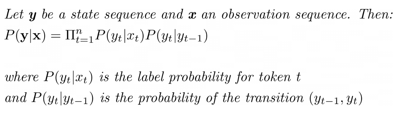
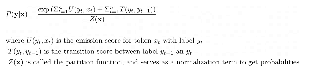
Since the input for NER tasks is a text (i.e a sequence of words), we can also turn the text into a linear chain (a simple directed graph where each word is a node, and there are vertices between contiguous words). Using a CRF, we can model the following conditional probability:
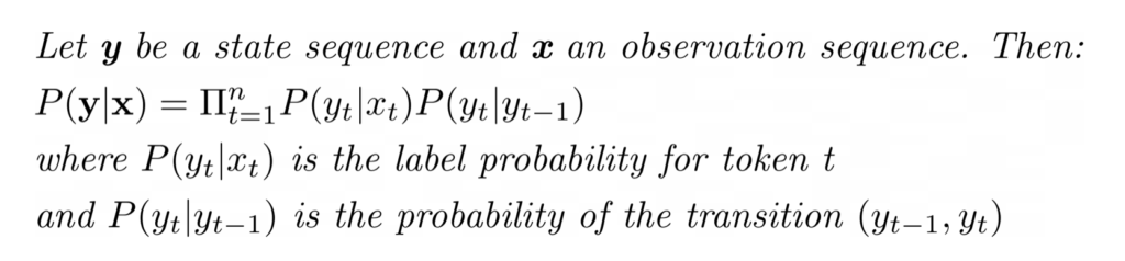
From the previous equation, you can see that we added a transition probability that accounts for the likelihood of observing each transition between labels in the sequence. This term will model the dependencies between the predictions of subsequent tokens, which is what we were missing in the previous formula.
[Author’s Note] conditioning on the previous label looks very similar to a Hidden Markov Model. I recommend reading this introduction to CRFs that explains in-depth the difference between HMM and CRF.
CRF-Layer for NER
For a typical NER Bi-LSTM+CRF model, the CRF layer is added right after the Bi-LSTM and takes the logits from the Bi-LSTM as inputs.
Let’s now examine how CRF layers are implemented in PyTorch.
CRF-layers are extremely light layers, and the only learned parameters is a k*k matrix that models the transition probabilities (the P(yt|xt) term).
Here is a screenshot of the Module init in the pytorch-crf repo:
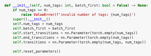
Source: pytorch-crf https://pytorch-crf.readthedocs.io/en/stable/
self.transitions is the k*k matrix of transitions probabilities and the main parameter from the CRF. self.start_transitions and self.end_transitions are added parameters corresponding to transitions specifically for the start and the end tokens.
For a NER model, a trained transition matrix could look like this:
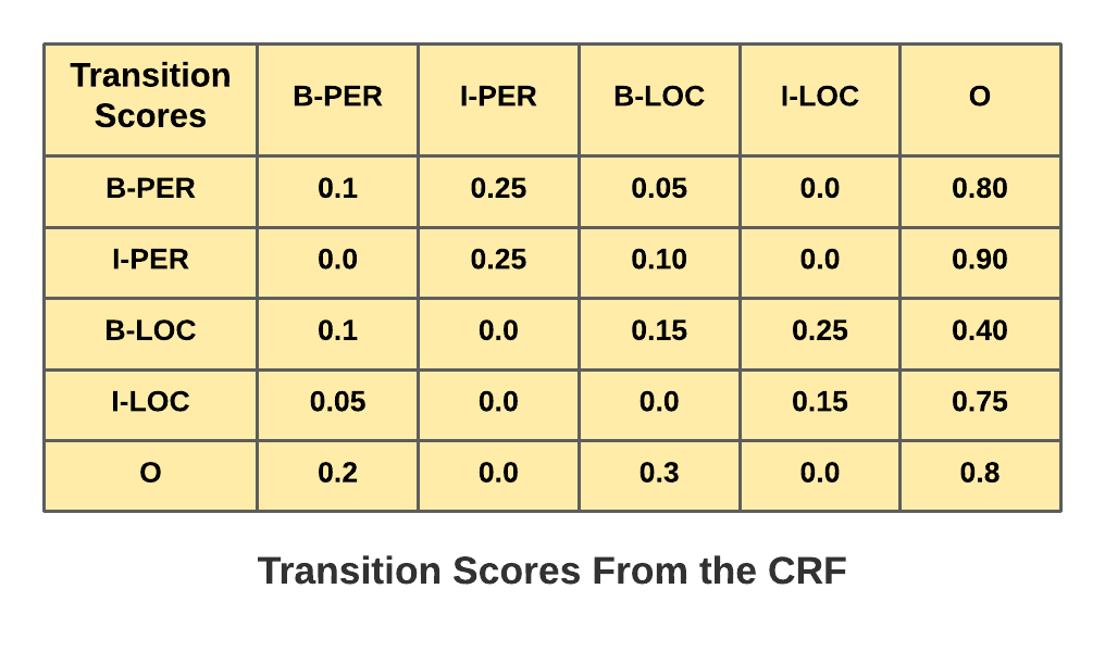
In this example, the transition score for [B-PER -> I-PER] is 0.25, whereas the transition score for [B-LOC -> I-PER] is 0.0. This reflects the fact that [B-PER -> I-PER] transitions are likely to happen, but [B-LOC, I-PER] should not occur, as that would be incorrect tagging.
[Author’s Note] You can hardcode some constraints into this matrix, by setting to 0.0 some transitions that are invalid for the task at hand.
CRF Loss and Decoding Procedure
We have seen in the previous section that the CRF adds a transition probability to the sequence probability, and the CRF layer needs to learn the transition matrix from the data. However, this is not the only difference.Two main issues arise:
- Greedy-decoding for inference can’t be used since there is an interaction between labels
- The cross-entropy loss for training is no longer viable since we now optimize over the sequence of tokens, not each token separately
Both need to be changed so that we can use the CRF in practice.
Conditional Probability in Exponential Form
The conditional probability of a sequence of labels is formulated as:
We can rewrite this probability in exponential form. We define U as the emission score function, T as the transition score function, and Z as the partition function, so that the conditional probability is:
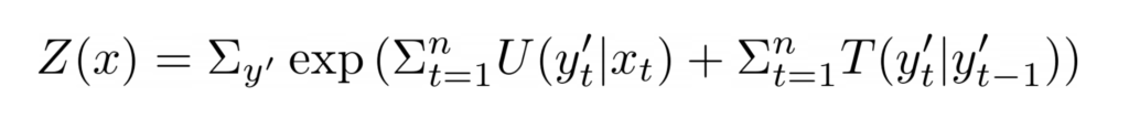
The partition function is a normalizing term. Since the numerator is a single sequence score, the partition function must be the sum of the scores of all possible sequences:
[Author’s Note] See this introduction on CRFs if you would like to learn more about this particular formulation of the conditional probability (involving feature functions). For the purpose of this blog post, we will skip the explanations.
CRF Loss
To train a CRF, we need a loss that optimizes the model so that the gold-label sequence (the ground truth) has a probability that tends to 1. That loss is obtained by computing the negative log-likelihood of the gold sequence (i.e the sequence from the ground truth) which is:
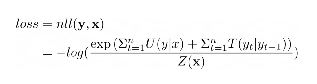
In the CRF loss, the numerator is the likelihood of the ground truth sequence. Since we have all emission and transition scores, it is trivial to calculate this likelihood given the labels.
However, computing the denominator (the partition function) is a lot more challenging since there is an exponential number of possible sequences (in the number of tokens in the sequence).
Computing the Partition Function with the Forward-Backward Algorithm
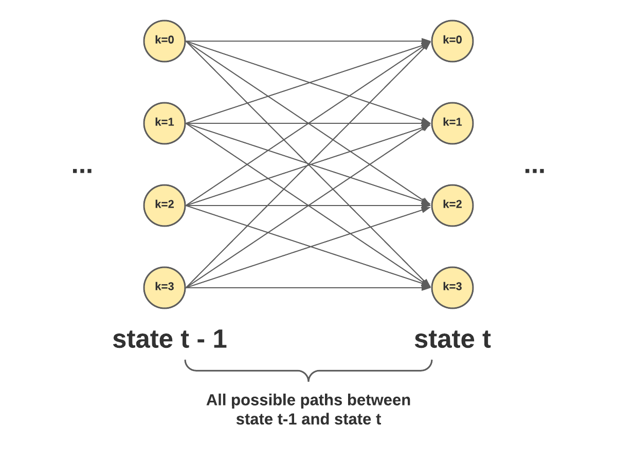
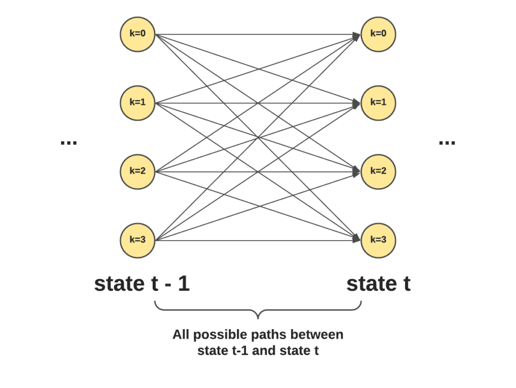
In this section, we will focus on the computation of the partition score, defined as the score of all possible paths given a series of observations.
The computational challenge is that there is an exponential number of possible paths (kN where k is the number of classes and N is the length of the sequence). Therefore, we cannot bluntly evaluate this function: it will have to be computed at each training and validation step so computational cost matters a lot.We need to find an efficient way of computing it.
The Forward-Backward Algorithm
Instead of computing the score for each possible path, we can leverage a recursive algorithm to do that: the forward-backward algorithm. By using dynamic programming, we can compute that partition function in 0(kN2).
The recursive formula is:
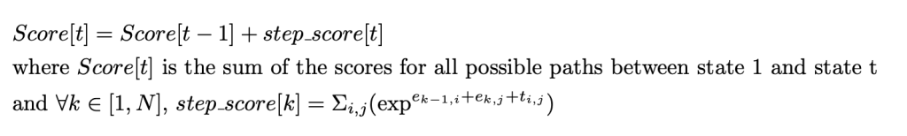
This can be read as:
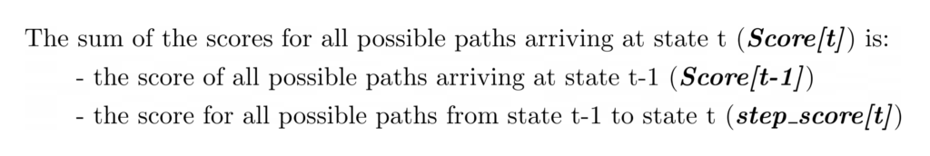
step_score can be seen as a “brute-force” computation of all possible transitions between t-1 and t and has a complexity of 0(kN). For each label, there are N potential transitions, and there are k labels in total.
Note that the step_score value is simple to evaluate since we have the emissions and transitions scores. Therefore, it’s just a matter of doing the sum of exponentials efficiently. And since we can dynamically build the Score values, we simply evaluate the step_score function at each step, hence the 0(kN2) complexity.
[Author’s Note] If you are interested to see some justifications for the recursion formula, I recommend looking at the following blog post that has the detailed computation of the first 3 steps of the forward-backward algorithm.
At Inference: Viterbi Algorithm
At inference time, we need to find the sequence with the highest probability (i.e the prediction). We now face a similar problem to the partition function: there is an exponential number of possible paths, and it is intractable to compute the likelihood of each path.
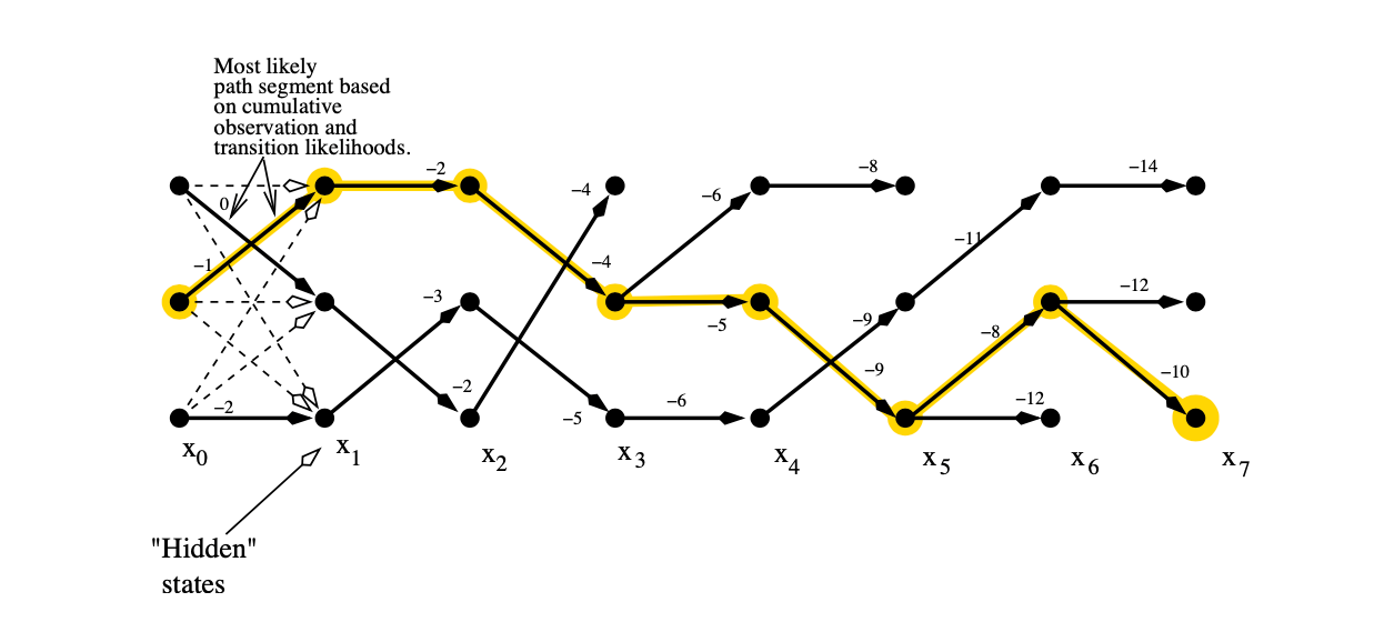
Source: The Viterbi Algorithm Demystified https://www.researchgate.net/publication/235958269_The_Viterbi_algorithm_demystified
Once again, there is a recursive algorithm that makes finding the highest probability path tractable: the Viterbi algorithm. The recursion formula is the following:
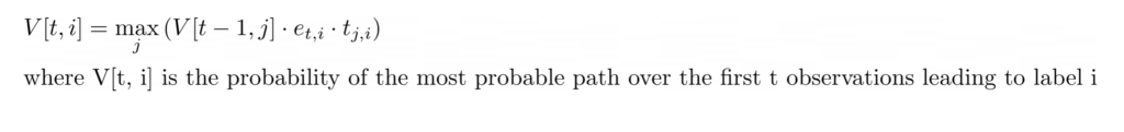
To get the best path (i.e highest likelihood sequence) leading to the token t having label i, we must:
- Find the best path to the previous token t-1 with label k (V[t-1,k])
- Multiply it with the emission score of token t with label i and transition score from k to i
- Maximize over k
Then, the sequence with the highest likelihood can be obtained by maximizing the score V for the last step of the sequence:
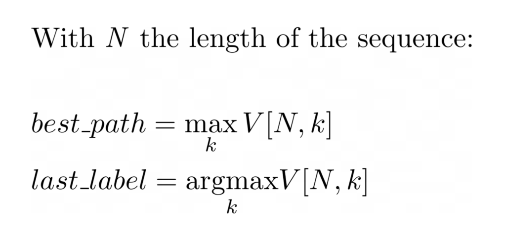
This gives the label of the final token for the highest likelihood sequence, and you can recover the labels of all the other tokens by back-tracking to the start of the sequence.
Although the forward-backward algorithm and the Viterbi algorithm have different recursive formulas, the idea is similar. We only need to compute the score/cost of going from state t-1 to state t, while re-using past results for all previous states.
CRF in the Context of Document Processing
As we have seen, linear-chain CRFs work with the assumption that we expect some dependencies between contiguous token labels. This assumption usually holds for sequences like texts. However, documents are by nature 2-dimensional, and automatically serializing a document is challenging. The most common technique for serialization is to extract line by line the text from the document, and this has a lot of limitations.
For instance, take this layout:
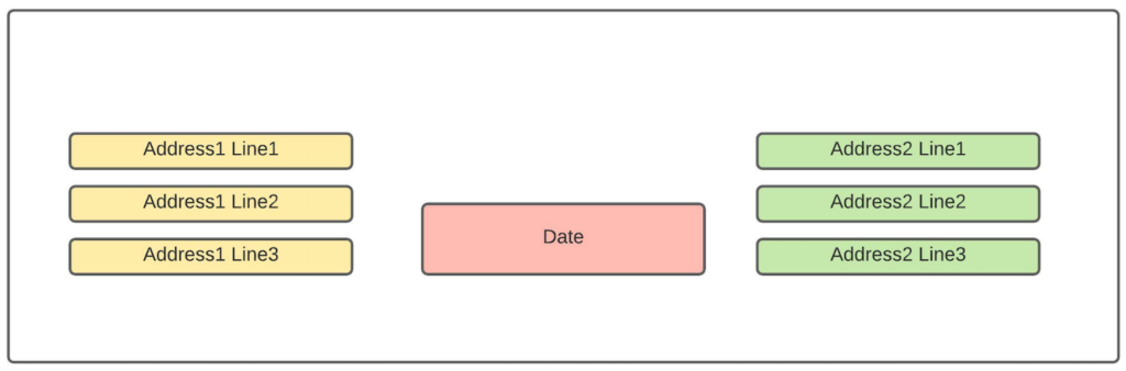
Automatically serializing the above content is challenging, as there are three separate columns with three separate lines. By serializing line by line, we would get the following:
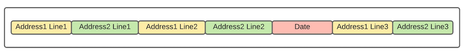
This sequence has several problems. First, we have broken down semantic blocks of text (the two addresses). Secondly, we have created noisy transitions between the tokens – notice the date is in the middle of 2 address lines. As a result, this sequence does not contain meaningful transitions. All transitions are nonsensical because the serialization was done improperly. Lastly, because those transitions are purely based on layout, they will randomly change from one layout to another, i.e the transitions will get even noisier. For that reason, it will be tricky for the CRF to model those transitions in a meaningful way.
Let’s say we “cheat” and manually compute a good serialization for the document:
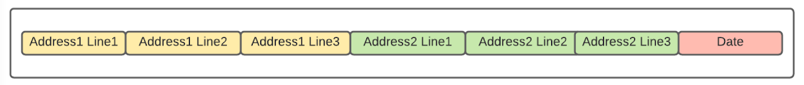
Even in that scenario, we have introduced at least 2 meaningless transitions: the transition between [Address1 Line3] and [Address2 Line1], and the transition between the [Address2 Line3] and [Date]. Those transitions are meaningless in the sense that they convey no information. You could have the date first, or the second address first, but it would not change any of the semantics for all the information here.
Therefore, when working on documents, the performance of the CRF is dependent on the layouts. The more unstructured the layouts are, the higher the expected performance.
Allowing Skip Connections
There is a variation on the Linear-chain CRF that allows for slightly more flexible graphs: the SkipChain CRF. As explained by Sutton and McCallum, you can slightly tweak a linear chain graph by defining rules to create (skip) connections between tokens that are not contiguous.
Source: An Introduction to Conditional Random Fields for Relational Learning https://people.cs.umass.edu/~mccallum/papers/crf-tutorial.pdf
However, this technique has mostly been used for some NLP tasks to aggregate information between multiple occurrences of the same word by using connections to get a more comprehensive context for the entity (see illustration above). There is no easy way to leverage those skip connections for documents, and as a result, most of the literature on sequence labeling for documents does not use CRFs.
In Summation
To sum up what we’ve learned from the CRF:
- It allows for optimizing over the entire sequence of labels rather than over each token label
- It is trained using the CRF loss that relies on the forward-backward algorithm
- At inference time, the Viterbi algorithm is used to compute the most probable sequence
This explains the unusual API from the pytorch-crf which was our starting point.
There are other well-established implementations available such as the allennlp implementation, but you can also check out this article to better understand how to efficiently implement such a mode.
Author’s Note: A big thanks to Johan Edvinsson and Pushkar Jain for their article review!